
As we explained in our previous post, Artificial Intelligence (AI) is more than Machine Learning (ML). Artificial Intelligence (AI) techniques include algorithms for finding optimal or pseudo-optimal solutions in complex problems, for example.
Several search problems can be described as a tree of options, in which each node of the tree is a partial or final solution to the problem and the branch below the node (if any), describes following options given that partial solution.
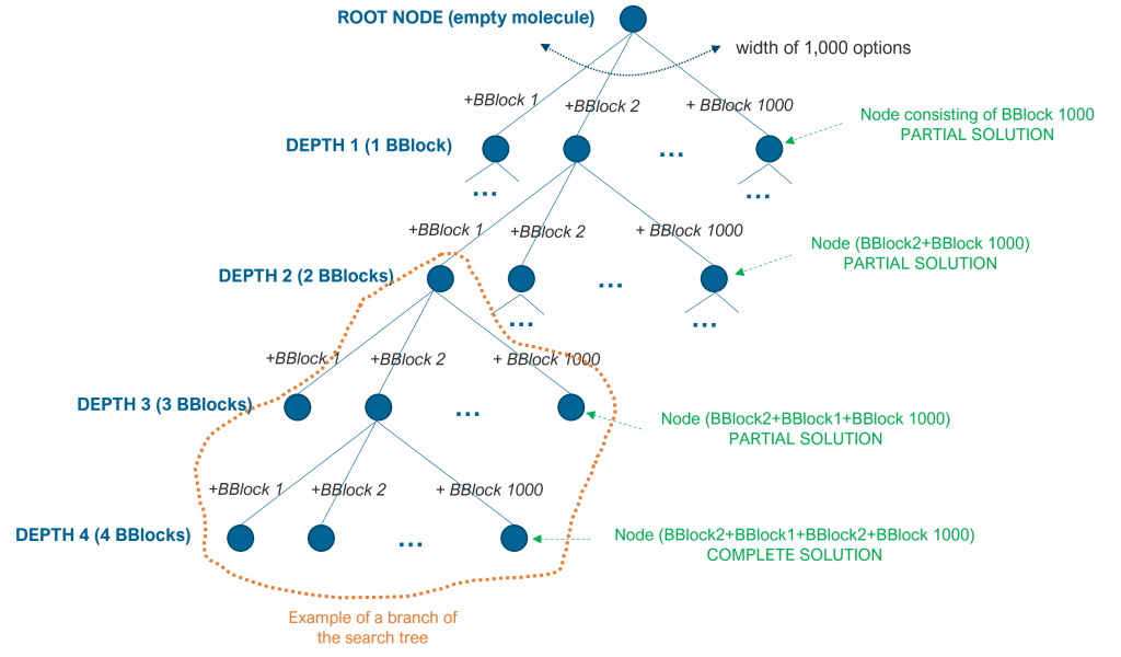
For instance, imagine we want to build a molecule by merging 4 building blocks from a pool of 1,000 blocks. For the sake of simplicity, let’s assume that building blocks can be combined in any form but two building blocks can only be combined in a single anchored point. The tree that describes the search space will have a root with an empty molecule (no building blocks) and a first level of nodes with width 1,000 (we can pick any building block as a starting point). A second level (depth) would consist of 1,000 nodes below each of the nodes in the first level: we can combine one building block with any of the 1,000 building blocks. And the same would happen for nodes in the 3rd and 4th levels (depths). Although this search tree has 4 depth levels given that we have described a constraint problem (4 building blocks), the search space is still enormous: 1,000^4 = 10^12.
As another example, the tree search space for a next chess game move is infinite. The root node of the tree describes the current situation of the pieces in the chess, each node below it describes a potential move of any of the existing pieces and so on for lower levels (depths). Each path from the root to any given node describes a series of potential moves (one white, one black). Since this is an unconstrained problem, search algorithms will limit the search space to an extent (e.g. a number of depths or next piece moves).
Note the importance of computing power to explore a large search space and to find better solutions in both cases in a reasonable amount of time.
Several algorithms exist for searching these tree spaces. These algorithms use a scoring function for each solution or partial solution to the problem (each tree node). In the case of molecules, it could be a Tanimoto-like score compared to a reference molecule. In the case of the chess game, it could be the difference between the number of existing pieces of the player taking the next move and the number of existing pieces of the opponent (evidently, this scoring is super simple, the one we used when we were kids).
Breadth-first search (BFS) algorithms explore first all the nodes of the current depth before exploring the nodes one depth lower. Depth-first search (DFS) algorithms, on the other hand, explore a given branch as deep as possible before backtracking up and following other branches. The following figure illustrates the search order to the molecular building blocks problem using BFS (in blue) and DFS (in green).
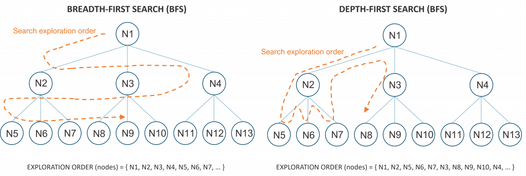
BFS algorithms require more memory than DFS algorithms, as the search space is explored in parallel and all options need to be kept in memory. DFS algorithms, on the other hand, are greedy algorithms that can get lost in a non-optimal branch if the search space is too big or infinite. Some DFS modifications tend to alleviate this problem by iteratively revisiting some of the top partial solutions and backtrack to other branches faster.
Several variants have been proposed to improve the time and memory requirements of these search algorithms. These variants mainly concentrate on two different aspects:
- Branch prioritization: by measuring or predicting that specific branches can lead to better solutions, the algorithm can explore these branches first and reach an optimal or pseudo-optimal solution faster.
- Branch pruning: by measuring or predicting that specific branches lead to poor solutions, the algorithm can prune those branches and skip exploring them.
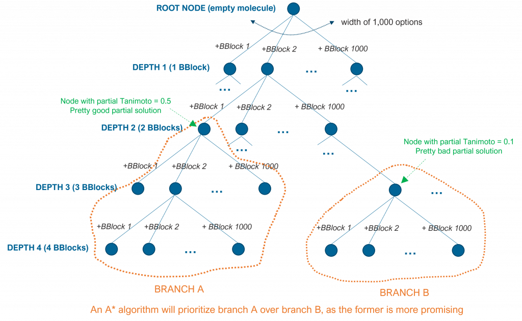
A* algorithms, for example, are best-first search algorithms. The idea of A* is to measure what is the score of a given internal node of the search tree and explore the subbranch that can potentially maximize the scoring function first. At each internal node, the algorithm computes the scoring function of that partial solution and it predicts or measures how far all the subbranches are to the optimal or pseudo-optimal solution.
For example, in the case of the molecular subblocks, the algorithm can prioritize a branch that starts at depth 2 with a Tanimoto value of 0.5 of that partial solution than a branch that starts at depth 3 with a Tanimoto value of 0.1. This is so because it is easier to find a better solution in the former, as depicted in the following figure.
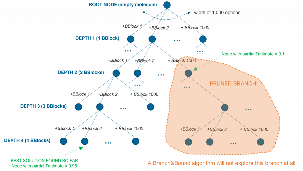
Branch and bound (BB or B&B) are also algorithms that prioritize some branches over others, but they also prune the search space by skipping specific branches that are computed to lead to suboptimal solutions. Such algorithms keep bounds or ranges of scoring values and they compute, at each internal node, if particular subbranches cannot lead to solutions that improve the best one found so far.
For simplicity, let’s assume that adding a building block can improve the current Tanimoto value of a partial solution in a range between 0 and 0.2. If the algorithm has already found a complete molecule of 4 building blocks that has a Tanimoto value of 0.95, it will not explore a subbranch at depth 2 if the Tanimoto value of that partial solution is 0.1. That partial solution can only be complemented by 2 building blocks and the best expected Tanimoto of any solution in that branch is 0.5 (the current 0.1 plus the maximum potential of +0.2 for each of the 2 final building blocks), as shown in the following figure.
The field of search algorithms, a fascinating component of Artificial Intelligence, is quite big and it has been widely studied. The basic algorithms described in this post date back from the 60s, 70s and 80s, with more modern variations in more recent years. I just wanted to provide a glimpse of some of the basic strategies. If interested, there are several books and papers around these topics.
Stay tuned for future post on other Artificial Intelligence posts.